SSD: Single Shot MultiBox Detector

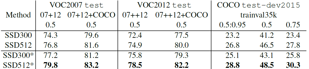
单阶段检测器，SSD300 achieves 74.3% mAP at 59 FPS while SSD500 achieves 76.9% mAP at 22 FPS。使用数据增强技巧后，SSD300 achieves 77.2% mAP while SSD500 achieves 79.8% mAP。

Overview

作为one-stage模型，SSD以VGG-16为主干网络，在不同尺度的feature maps下进行辨别的工作，这样的机制被称为 Pyramidal Feature Hierarchy。

SSD overview

MultiBox Detector

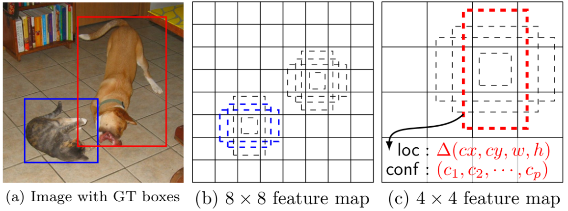
a) After going through a certain of convolutions for feature extraction, we obtain a feature layer of size m×n (8×8 or 4×4) with P channels. And a 3×3 conv is applied on this m×n×p feature layer.

b) For each location, we got k bounding boxes. These k bounding boxes have different sizes and aspect ratios.

c) For each of the bounding box, we will compute c class scores and 4 offsets relative to the original default bounding box shape.Thus, we got (c+4)xkmn outputs.

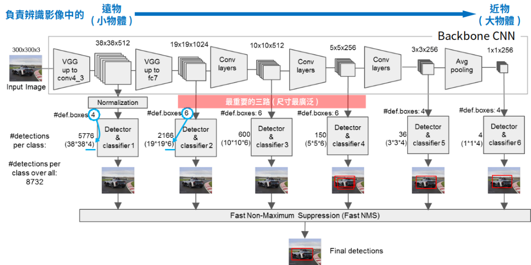
SSD300 Network Architecture

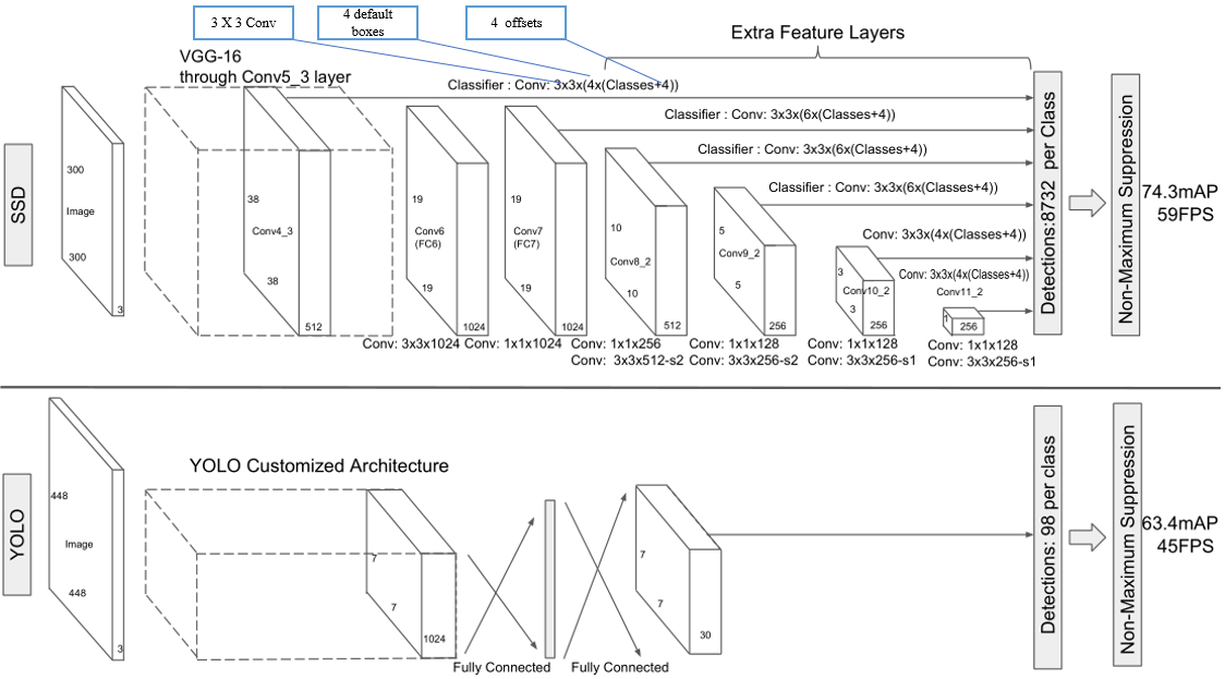
At Conv4_3, it is of size 38×38×512 and 3×3 conv is applied. And there are 4 bounding boxes and each bounding box will have (classes + 4) outputs. Thus, at Conv4_3, the output is 38×38×4×(c+4). Suppose there are 20 object classes plus one background class, the output is 38×38×4×(21+4) = 144,400. In terms of number of bounding boxes, there are 38×38×4 = 5776 bounding boxes.

a) Conv4: 38×38×4 = 5776 boxes (4 boxes for each location)

b) Conv7: 19×19×6 = 2166 boxes (6 boxes for each location)

c) Conv8_2: 10×10×6 = 600 boxes (6 boxes for each location)

d) Conv9_2: 5×5×6 = 150 boxes (6 boxes for each location)

e) Conv10_2: 3×3×4 = 36 boxes (4 boxes for each location)

f) Conv11_2: 1×1×4 = 4 boxes (4 boxes for each location)

There are 5776 + 2166 + 600 + 150 + 36 +4 = 8732 boxes in total

取出feature map之后，SSD通过一次3×3的卷积得到用于detector的神经层。而卷积的深度就是与default box有关。若假定default box数量为D，而目标类别有C个类别，边界框有4个值(x，y，w，h)的偏差量(offsets)，所以深度的计算就是D×(4+C)。

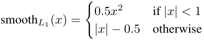
Loss Function

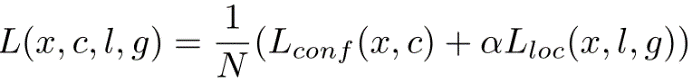
The loss function consists of two terms: L~~conf~~ and L~~loc~~ where N is the matched default boxes.

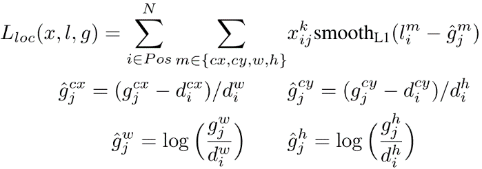
Localization Loss

L~~loc~~ is the localization loss which is the smooth L1 loss between the predicted box (l) and the ground-truth box (g) parameters. These parameters include the offsets for the center point (cx, cy), width (w) and height (h) of the default bounding box. This loss is similar to the one in Faster R-CNN.

Smooth L1

Confidence Loss

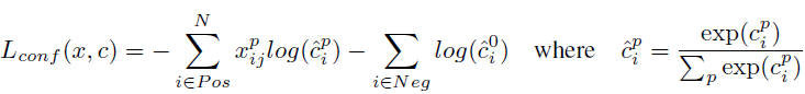
L~~conf~~ is the confidence loss which is the softmax loss over multiple classes confidences (c). (α is set to 1 by cross validation.).

Scales and Aspect Ratios of Default Boxes

Scale of default boxes

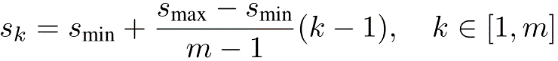
Suppose we have m feature maps for prediction, we can calculate Sk for the k-th feature map. S~~min~~ is 0.2, S~~max~~ is 0.9. That means the scale at the lowest layer is 0.2 and the scale at the highest layer is 0.9. All layers in between is regularly spaced.

For each scale, SK, we have 5 non-square aspect ratios:

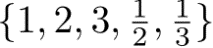
For aspect ratio of 1:1, we got Sk^’^:

Therefore, we can have at most 6 bounding boxes in total with different aspect ratios. For layers with only 4 bounding boxes, ar = 1/3 and 3 are omitted.

Details of Training

Hard Negative Mining

Instead of using all the negative examples, we sort them using the highest confidence loss for each default box and pick the top ones so that the ratio between the negatives and positives is at most 3:1.This can lead to faster optimization and a more stable training.

Data Augmentation

Each training image is randomly sampled by:

a) entire original input image

b) Sample a patch so that the overlap with objects is 0.1, 0.3, 0.5, 0.7 or 0.9.

c) Randomly sample a patch

The size of each sampled patch is [0.1, 1] or original image size, and aspect ratio from 1/2 to 2.After the above steps, each sampled patch will be resized to fixed size and maybe horizontally flipped with probability of 0.5, in addition to some photo-metric distortions.

Atrous Convolution (Hole Algorithm / Dilated Convolution)

The base network is VGG16 and pre-trained using ILSVRC classification dataset. FC6 and FC7 are changed to convolution layers as Conv6 and Conv7. Furthermore, FC6 and FC7 use Atrous convolution (Hole algorithm or dilated convolution) instead of conventional convolution. And pool5 is changed from 2×2-s2 to 3×3-s1**.**

参考博客：[https://towardsdatascience.com/review-ssd-single-shot-detector-object-detection-851a94607d11]{.underline}

简单例子，普通卷积3*3计算一个值，空洞卷积5*5计算一个值

The feature maps are large at Conv6 and Conv7, using Atrous convolution as shown above can increase the receptive field while keeping number of parameters relatively fewer compared with conventional convolution.

Results

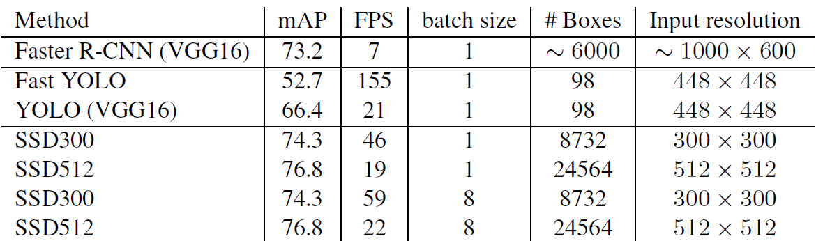
There are two Models: SSD300 and SSD512. SSD300: 300×300 input image, lower resolution, faster. SSD512: 512×512 input image, higher resolution, more accurate.

Model Analysis

Model analysis

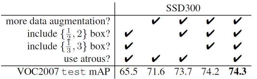
a) Data Augmentation is crucial, which improves from 65.5% to 74.3% mAP.

b) With more default box shapes, it improves from 71.6% to 74.3% mAP.

c) With Atrous, the result is about the same. But the one without atrous is about 20% slower.

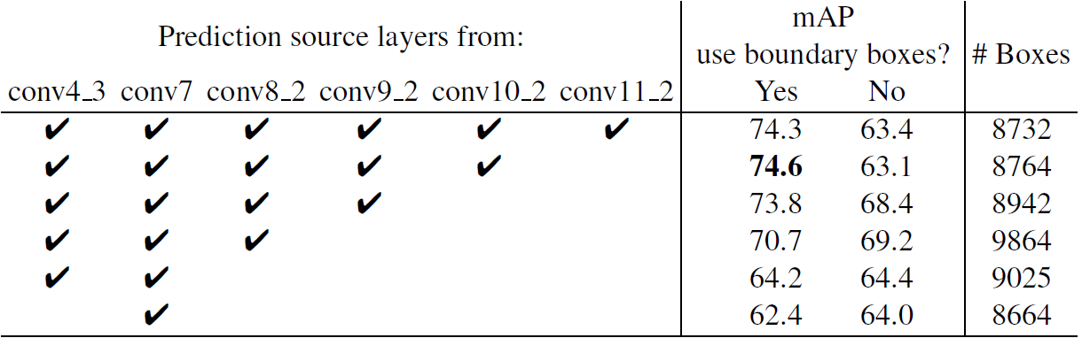
Multiple output layers at different resolutions

是否使用使用boundry boxes? ---- 是否剔除超出边界的bbox

With more output from conv layers, more bounding boxes are included. Normally, the accuracy is improved from 62.4% to 74.6%. However, the inclusion of conv11_2 makes the result worse. Authors think that boxes are not enough large to cover large objects.

PASCAL VOC 2007

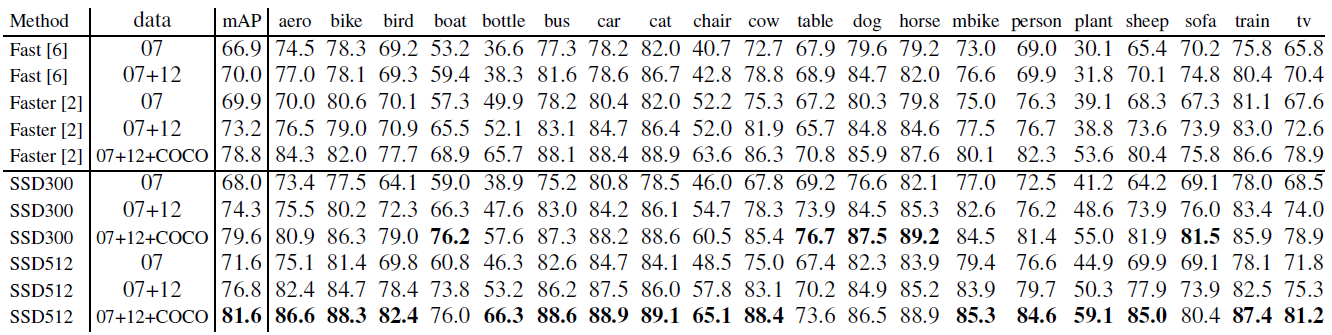
Detetcion results on PASCAL VOC2007

a) 更多的训练图片带来更好的检测准确率

b) SSD512有68.0%的mAP 并且SSD300有71.6% mAP 都优于Faster R-CNN的69.9%mAP.

PASCAL VOC 2012

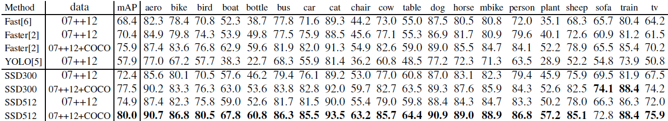
Detection Results on PASCAL VOC2012

MS COCO

Detection results on MS COCO

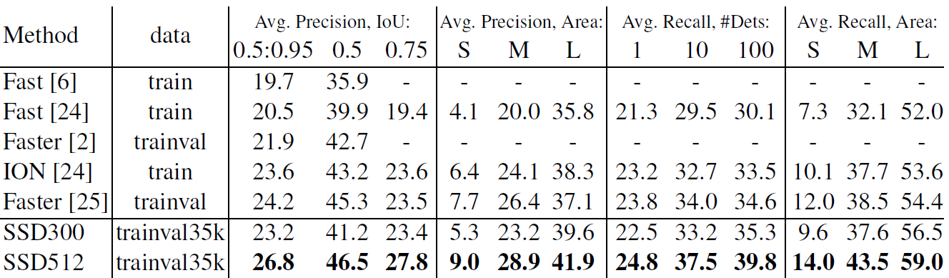
a) SSD512 is only 1.2% better than Faster R-CNN in mAP@0.5. This is because it has much better AP (4.8%) and AR (4.6%) for larger objects, but has relatively less improvement in AP (1.3%) and AR (2.0%) for small objects.

b) Faster R-CNN is more competitive on smaller objects with SSD. Authors believe it is due to the RPN-based approaches which consist of two shots(在RPN阶段和分类预测都有offset调整).

Data Augmentation for Small Object Accuracy

To overcome the weakness of missing detection on small object as mentioned in 6.4, “zoom out” operation is done to create more small training samples.And an increase of 2%-3% mAP is achieved across multiple datasets as shown below: